Contents

• Description of MercPert
• Using MercPert
• Suggestions for playing with MercPert
• Understanding MercPert
• Suggested modifications of MercPert
• Listing of the Java code for MercPert

Description of MercPert

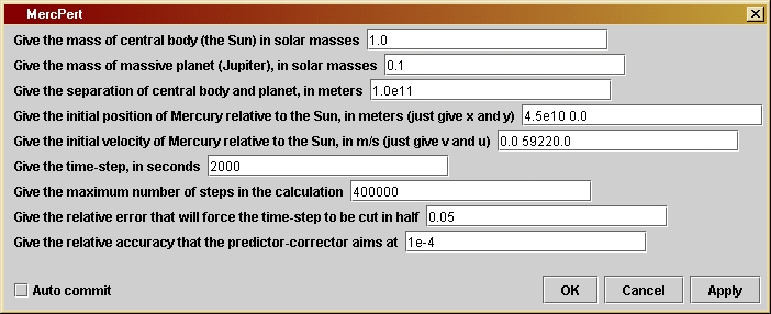
The user can choose the masses and separation of the binary bodies, the initial condition and location of the smaller planet, and the same parameters that govern the program as in previous orbit programs like Orbit and Binary: time-step length, number of time-steps, and the accuracy parameters for time-step halving and for the predictor-corrector method.

MercPert is our first look at the complex world of systems containing more than two bodies. We are starting gently here, by studying a special case. As explained in Chapter 13, only the gravity produced by the binary system is taken into account: the small "Mercury" is assumed to have negligible effect on the other two bodies. (Physicists call this the "restricted three-body problem", restricted because the mass of the third body is negligible.) The binary system, moreover, has a circular orbit, and "Mercury" will move only in the plane of this orbit. This special case is nevertheless very interesting, not only for the amaxing complexity of the effects on "Mercury" but also because this situation is duplicated in many young solar systems, where massive planets like this super-Jupiter clear out a region of the proto-planetary disk and prevent other planets from forming nearby.

Using MercPert

You can change the parameters by opening up the parameter window: double-click on the unit's icon when it is in the working area to get a window like the one shown to the left. The default parameters represent a situation that will evolve roughly like Figure 13.4 of the book, where "Mercury" is attracted by "Jupiter" and loops once around it backwards, winding up on a tighter and more eccentric orbit around the Sun. The first parameter allows the user to choose the mass of one of the binary bodies (conventionally, the "Sun", but it need not even be the more massive of the two), and the second parameter is for the mass of the second binary body ("Jupiter"). Both masses are given in solar masses, not in kg. The third parameter is the separation of the binary bodies, in meters. Since the program assumes they are in a circular binary orbit, giving their separation and their masses fixes the binary system completely. The program assumes that at the initial moment, the binary bodies lie on the x-axis, with the first body at negative-x and the second at positive-x. Their orbits follow circles in the counter-clockwise direction, and the centers of both circles remain at the origin of the coordinates. This information is important for deciding where to place the third body ("Mercury"). Its initial position is given in the fourth line: the user should type both coordinates (in meters), separated by one or more spaces, but without additional punctuation. Similarly, the user should type into the fifth line the initial velocity of "Mercury", again giving both components separated by spaces (in meters per second). This fully determines the orbit of the third body. The remaining parameters are similar to those in Orbit and Binary that control the running of the program: time-step length, number of time-steps, and two accuracy parameters.

One difference with previous programs is that this one does not stop once "Mercury" has made a complete orbit. The trajectory of Mercury can be so irregular that this criterion would be meaningless; moreover, it is very interesting to watch the system evolve over many orbits. So the only thing that stops the program is reaching the total number of time-steps given in the seventh parameter. Notice that the total elapsed time along the orbit is not predictable, since the time-step can be reduced by the program. Just experiment with the program and if it does not go as far as you want, reset the number of time-steps to a larger number and run it again. Notice also that there is no choice-box offering you different output options. For this program only the orbits are output.

Suggestions for playing with MercPert

There are a few things that you should notice in these examples.

• "Mercury" often has more than one very close encounters with "Jupiter". An "encounter" is not just a place where orbits cross, since the two bodies may not have been in the same places in their orbits at the time of the crossing. You can see where a genuine encounter happens by looking for sharp changes in the trajectory of "Mercury". In the fifth simulation there are at least five close encounters.
• These encounters tend to put "Mercury" into a highly eccentric orbit that takes it close to the "Sun". These are good examples of what we called "slinging toward the Sun" in Chapter 6.  In several of the simulations, "Mercury" comes so close to the "Sun" that, if we were to allow for the finite size of the central star, we would expect it to be swallowed by the "Sun" and removed from the planetary system. This is the principal mechanism for the cleaning out of a proto-solar-system. Notice, however, that in three simulations, "Mercury" is expelled from the system entirely after its close encounter with the Sun.
• Just for fun we ran one orbit where "Mercury" began very close to "Jupiter" (the fifth image). It is immediately captured and becomes a moon of "Jupiter".
• In the final simulation, "Mercury" is started out in a retrograde orbit, one which circles the "Sun" in the opposite sense from "Jupiter's". This remains stable, because "Mercury" never spends enough time near "Jupiter" to be seriously disturbed.
  

This program can simulate a much larger variety of systems than just Sun+Jupiter. Because you can choose the initial masses and separations of the binary bodies freely, you can explore many other kinds of systems. Try the following:

• Equal-mass binary. Set the two masses equal to 1 and set the separation to about 1 AU. This represents a fairly typical binary system with solar-type stars. Can you find any orbits between the two bodies that are stable? Can you find stable orbits that stay far outside the binary orbit? Would, say, a planet at Jupiter's distance from the Sun remain in orbit for a long time around this system?
• The Roche limit. Set the two masses equal to 10 and 1 and set the separation to about 0.3 AU. This represents a typical binary containing a black hole (10 solar masses) and an ordinary solar-mass star, with a moderate separation. Now experiment with orbits for the small body that might tell us about the way the black hole strips gas from the normal star. This gas starts out at the surface of the solar-mass star, which might be a good fraction of the distance between the hole and the star if the star has become a giant. The gas starts out at rest with respect to the binary system, which means it moves with the same initial angular velocity as the star and black hole. Compute this angular velocity and use it to set up initial data as follows. Take the initial x-position to be anywhere you like between the two bodies. Take the initial y-position to be zero. Take the initial x-velocity to be zero and the initial y-velocity to be the angular velocity times the x-position. By changing the initial position, find out what possible behaviors there are. For what range of starting positions does the small body fall toward the black hole? For what positions does it remain near the star? The dividing place is called the Roche limit: if a giant star in a binary expands to larger than this size, it will lose its outer layers, which will fall onto the black hole. Note that what happens to gas and to our small body when they fall toward the black hole will be very different: the small body will just follow a gravitational trajectory, but the gas will get hot, develop strong pressure gradients, and radiate away much of its energy. The gas will then be trapped into an accretion disk around the black hole. See the discussion of accretion disks in Chapter 13. But even though the subsequent motion of gas and small particles will be different, the Roche limit will be the same, because at the outer edge of a star the pressure is zero so the gas particles behave like freely orbiting bodies.

Understanding MercPert

In the program, variables relating to the "Sun" have names ending in Sun, those relating to "Jupiter" have names ending in Planet, and those relating to "Mercury" have names including the word Merc.

The positions of the binary bodies do not need to be calculated from their accelerations.We already know how a circular binary moves, so we can just write down their positions at any time. We know from the discussion in Invesigation 13.1 that they have orbital radii in inverse proportion to their masses, so that we can calculate at the beginning of the program the orbital radius of the "Sun", rSun, from the two binary masses mSun and mPlanet and their separation binarySeparation, all three of which are given by the user in the parameter window:
        double rSun = mPlanet/(mSun + mPlanet)*binarySeparation;
Then the radius of "Juptier's" orbit must make up the remainder of the separation of the two bodies:
        double rPlanet = binarySeparation - rSun;
The bodies orbit each other with the angular velocity omega that one can deduce from Equation 13.4 by solving for 2p/P, where P is the orbital period:
        double omega = Math.sqrt(kGravity*(mSun + mPlanet)/Math.pow(binarySeparation,3));
Recall that, as in the program Binary, kGravity is the product of Newton's gravitational constant G and the mass of the Sun. This allows us to use the variables mSun and mPlanet for the masses of these bodies in units of solar masses.

Given these variables, then at any time t the coordinate positions of the binary bodies are
        xSun = -rSun*Math.cos(omega*t);
        ySun = -rSun*Math.sin(omega*t);
        xPlanet = rPlanet*Math.cos(omega*t);
        yPlanet = rPlanet*Math.sin(omega*t);
The minus signs in the first two expressions reflect the fact that the "Sun's" initial position is on the negative-x-axis. In fact, you will not see lines like these explicitly in the code below. Instead, it is more efficient to compute the sine and cosine just once, assigning their values to variables s1 and c1, respectively. Moreover, there are no variables xSun, ySun, ..., in the program because the only thing that is important is the distance of "Mercury" from the binary bodies. Therefore what one finds in the code instead of the above are lines like
        c1 = Math.cos(t1*omega);
        s1 = Math.sin(t1*omega);
        xMercSun1 = xMerc1 + rSun * c1;
        yMercSun1 = yMerc1 + rSun * s1;
        xMercPlanet1 = xMerc1 - rPlanet * c1;
        yMercPlanet1 = yMerc1 - rPlanet * s1;
which compute the components of the displacement vectors from the binary bodies to "Mercury".

As in previous programs, once this displacement is known the acceleration of "Mercury" can be computed, as the sum of the accelerations produced by the two binary bodies. This is done in program lines like
        rMercSun = Math.sqrt( xMercSun1*xMercSun1 + yMercSun1*yMercSun1 );
        rMercSun3 = Math.pow(rMercSun,3);
        rMercPlanet = Math.sqrt( xMercPlanet1*xMercPlanet1 + yMercPlanet1*yMercPlanet1 );
        rMercPlanet3 = Math.pow(rMercPlanet,3);
        axMerc1 = -kGravity * ( mSun*xMercSun1/rMercSun3 + mPlanet*xMercPlanet1/rMercPlanet3 );
        ayMerc1 = -kGravity * ( mSun*yMercSun1/rMercSun3 + mPlanet*yMercPlanet1/rMercPlanet3 );
These should be self-explanatory, if you have followed the development of Binary. From these acceleration components the program computes the orbit of "Mercury" in the usual way.

The remaining parts of the program are the same as before, with time-step halving and the predictor-corrector. The loop that moves forward in time is even simpler, since there is no test for the completion of one orbit: it just runs until it reaches the maximum number of steps set by the user.
 

Suggested modifications of MercPert

If you want to change the program you will have to re-compile it, as explained by the help file Using Triana for Gravity from the ground up.
 

Listing of the Java code for MercPert

Preliminary definitions of parameters and constants

    /*
      binarySeparation is the distance between the central body and the
      planet, both of which are taken to follow circular orbits. They
      begin at t=0 with a separation just along the x-direction. The
      separation is in meters and is set by the user in the parameter
      window.
      */
    private double binarySeparation;
 

    /*
      initPosMerc is the String used by the program to allow users
      to input the initial position of "Mercury" in the parameter
      window. The String is processed to obtain the initial x-
      and y-positions, which are stored in xInitMerc and yInitMerc.
      All positions are given in meters.
    */
    private String initPosMerc;
    private double xInitMerc;
    private double yInitMerc;

    /*
    initVelMerc is the String used by the program to allow users
    to input the initial velocity of "Mercury" in the parameter
    window. The String is processed to obtain the initial x-
    and y-velocity components, which are stored in vInitMerc
    and uInitMerc. All velocities are given in m/s.
    */
    private String initVelMerc;
    private double vInitMerc;
    private double uInitMerc;

    /*
      dt is the time-step in seconds. It is set by the user in the
      parameter window.
    */
    private double dt;

    /*
      maxSteps is the maximum number of steps in the calculation.
      This is used to ensure that the calculation will stop even
      if initial values are chosen so that "Mercury" is expelled
      from the Solar System. It is set by the user in the parameter
      window.
    */
    private int maxSteps;

    /*
      eps1 sets the accuracy of the time-step. If computed quantities
      change by a larger fraction than this in a time-step, the time-step
      will be cut in half, repeatedly if necessary. It is set by the user
      in the parameter window.
    */
    private double eps1;

    /*
      eps2 sets the accuracy of the predictor-corrector step. Averaging
      over the most recent time-step is iterated until it changes by
      less than this relative amount. It is set by the user in the
      parameter window.
    */
    private double eps2;

    /*
      kGravity is Newton's gravitational constant times the mass of the Sun.
      It is used internally and not set by the user.
    */
    private double kGravity = 1.327e20;
 
 

Program code

        /*
          Now define other variables that will be needed, but without giving
          initial values. They will be assigned values during the calculation.
          - t1 is a temporary value of the time, used to compute postions of the
            binary bodies when needed.
          - xMerc1 and yMerc1 are temporary values of x and y for Mercury that are
            needed during the calculation.
          - axMerc1 and ayMerc1 are likewise temporary values of the acceleration.
          - dxMerc and dyMerc are variables that hold part of the changes in
            x and y for Mercury that occur during a time-step.
          - ddxMerc0, ddxMerc1, ddyMerc0 and ddyMerc1 are variables that hold other parts of
            the changes in x and y of Mercury during a time-step. The reason for having
            both dxMerc and ddxMerc will be explained in comments on the calculation below.
          - dvMerc and duMerc are the changes in velocity components of Mercury that occur
            during a time-step.
          - xMercSun1, yMercSun1, xMercPlanet1, and yMercPlanet1 are temporary values that
            hold the separations of Mercury from the Sun and the massive planet, respectively.
          - testPrediction will hold a value that is used by the predictor-corrector
            steps to assess how accurately the calculation is proceeding.
          - c1 and s1 are temporary variables used to make the computation of the positions
            of the Sun and the massive planet more efficient.
          - j and k are integers that will be used as loop counters.
        */
        double t1, xMerc1, yMerc1, axMerc1, ayMerc1, dvMerc, duMerc;
        double dxMerc, dyMerc, ddxMerc0, ddyMerc0, ddxMerc1, ddyMerc1;
        double xMercSun1, yMercSun1, xMercPlanet1, yMercPlanet1;
        double testPrediction;
        double c1, s1;
        int j, k;

        /*
          Now start the loop that computes the two orbits. The loop counter
          is j, which (as in Orbit) starts at 1 and increases by 1 each
          step. The test for exiting from the loop will be that the number
          of steps exceeds  the maximum set by the user.
        */
        for ( j = 1; j < maxSteps ; j++ ) {

            /*
              - Set dvMerc and duMerc to the changes in x- and y-speeds that would occur
                during time dt1 if the acceleration were constant at (axMerc0, ayMerc0).
              - Similarly set dxMerc and dyMerc to the changes in position that would
                occur if the velocity components vMerc and uMerc were constant during the
                time dt1.
              - Set ddxMerc0 and ddyMerc0 to the extra changes in x and y that occur because
                Mercury's velocity changes during the time dt1. The velocity change that
                is used is only dvMerc/2 (or duMerc/2, respectively) because the most
                accurate change in position comes from computing the average
                velocity during dt1. We separate the two position changes, dxMerc and
                ddxMerc0, because dxMerc will be unchanged when we do the predictor-corrector
                below (the change in position due to the original speed is always
                there), while ddxMerc0 will be modified when axMerc0 and hence dvMerc is modified
                by the predictor-corrector.
              - Finally, set ddxMerc1 and ddyMerc1 to ddxMerc0 and ddyMerc0 initially. They will
                change when we enter the predictor-corrector code.
            */
            t1 = t + dt1;
            dvMerc = axMerc0*dt1;
            duMerc = ayMerc0*dt1;
            dxMerc = vMerc*dt1;
            dyMerc = uMerc*dt1;
            ddxMerc0 = dvMerc/2*dt1;
            ddyMerc0 = duMerc/2*dt1;
            ddxMerc1 = ddxMerc0;
            ddyMerc1 = ddyMerc0;

            /*
              Now advance the position of Mercury by our initial estimates of the
              position changes, dxMerc + ddxMerc0 and dyMerc + ddyMerc0. Then
              compute the new distances of Mercury from the binary bodies and the
              resulting acceleration at this position. Use the positions of the
              binary bodies at the time t1.
            */
            xMerc1 = xMerc0 + dxMerc + ddxMerc0;
            yMerc1 = yMerc0 + dyMerc + ddyMerc0;
            c1 = Math.cos(t1*omega);
            s1 = Math.sin(t1*omega);
            xMercSun1 = xMerc1 + rSun * c1;
            yMercSun1 = yMerc1 + rSun * s1;
            rMercSun = Math.sqrt( xMercSun1*xMercSun1 + yMercSun1*yMercSun1 );
            rMercSun3 = Math.pow(rMercSun,3);
            xMercPlanet1 = xMerc1 - rPlanet * c1;
            yMercPlanet1 = yMerc1 - rPlanet * s1;
            rMercPlanet = Math.sqrt( xMercPlanet1*xMercPlanet1 + yMercPlanet1*yMercPlanet1 );
            rMercPlanet3 = Math.pow(rMercPlanet,3);
            axMerc1 = -kGravity * ( mSun*xMercSun1/rMercSun3 + mPlanet*xMercPlanet1/rMercPlanet3 );
            ayMerc1 = -kGravity * ( mSun*yMercSun1/rMercSun3 + mPlanet*yMercPlanet1/rMercPlanet3 );

            /*
              Time-step check.
              This is the code to check whether the time-step is too large. The idea
              is to compare the changes in acceleration of Mercury during the timestep
              with the acceleration of Mercury itself. If the change is too
              large a fraction of the original value, then the step is likely to be
              too large, and the resulting position too inaccurate. The code below cuts
              the time-step dt1 in half and then goes back to the beginning of the loop.
              This is explained more fully in the program Orbit.
            */
            if ( Math.abs(axMerc1-axMerc0) + Math.abs(ayMerc1-ayMerc0) > eps1*(Math.abs(axMerc0) + Math.abs(ayMerc0)) ){
                dt1 /= 2;
                j--;
            }
            else {

                /*
                  Predictor-corrector step. This is explained in program Orbit.
                */
                testPrediction = Math.abs(ddxMerc0) + Math.abs(ddyMerc0);
                for ( k = 0; k < 10; k++ ) {
                    /* compute dvMerc and duMerc by averaging the acceleration over dt1 */
                    dvMerc = (axMerc0 + axMerc1)/2*dt1;
                    duMerc = (ayMerc0 + ayMerc1)/2*dt1;
                    /* compute ddxMerc1 and ddyMerc1 by averaging the velocity change */
                    ddxMerc1 = dvMerc/2*dt1;
                    ddyMerc1 = duMerc/2*dt1;

                    /*
                      Test the change in ddx and ddy since the last iteration.
                      If it is more than a fraction eps2 of the original, then
                      ddx and ddy have to be re-computed by finding the acceleration
                      at the refined position.
                      If the change is small enough, then the "else:" clause is
                      executed, which exits from the for loop using the statement
                      "break". This finishes the iteration and goes on to wrap up
                      the calculation.
                    */
                    if ( Math.abs(ddxMerc1-ddxMerc0) + Math.abs(ddyMerc1-ddyMerc0) > eps2 * testPrediction ) {
                        /*
                          Re-define ddxMerc0 and ddyMerc0 to hold the values
                          from the last iteration
                        */
                        ddxMerc0 = ddxMerc1;
                        ddyMerc0 = ddyMerc1;
                        xMerc1 = xMerc0 + dxMerc + ddxMerc0;
                        yMerc1 = yMerc0 + dyMerc + ddyMerc0;
                        c1 = Math.cos(t1*omega);
                        s1 = Math.sin(t1*omega);
                        xMercSun1 = xMerc1 + rSun * c1;
                        yMercSun1 = yMerc1 + rSun * s1;
                        rMercSun = Math.sqrt( xMercSun1*xMercSun1 + yMercSun1*yMercSun1 );
                        rMercSun3 = Math.pow(rMercSun,3);
                        xMercPlanet1 = xMerc1 - rPlanet * c1;
                        yMercPlanet1 = yMerc1 - rPlanet * s1;
                        rMercPlanet = Math.sqrt( xMercPlanet1*xMercPlanet1 + yMercPlanet1*yMercPlanet1 );
                        rMercPlanet3 = Math.pow(rMercPlanet,3);
                        axMerc1 = -kGravity * ( mSun*xMercSun1/rMercSun3 + mPlanet*xMercPlanet1/rMercPlanet3 );
                        ayMerc1 = -kGravity * ( mSun*yMercSun1/rMercSun3 + mPlanet*yMercPlanet1/rMercPlanet3 );

                        /*
                          We now have the "best" acceleration values, using the most
                          recent estimates of the position at the end of the loop.
                          The next statement to be executed will be the first statement
                          of the "for" loop, finding better values of dvMerc, duMerc, ddxMerc1,
                          and ddyMerc1.
                        */
                    }
                    else break;
                }

                /*
                  The iteration has finished, and we have sufficiently accurate
                  values of the position change in ddxMerc1 and ddyMerc1.
                  Use them to get final values of xMerc and yMerc at the end of
                  the time-step dt1 and store these into xMerc0 and yMerc0,
                  respectively, ready for the next time-step. Compute all the
                  rest of the variables needed for the next time-step and for
                  possible data output.
                */
                t += dt1;
                xMerc0 += dxMerc + ddxMerc1;
                yMerc0 += dyMerc + ddyMerc1;
                axMerc0 = axMerc1;
                ayMerc0 = ayMerc1;
                vMerc += dvMerc;
                uMerc += duMerc;
                xCoordinateMerc[j] = xMerc0;
                yCoordinateMerc[j] = yMerc0;
                c1 = Math.cos(t * omega);
                s1 = Math.sin(t * omega);
                xCoordinateSun[j] = -rSun*c1;
                yCoordinateSun[j] = -rSun*s1;
                xCoordinatePlanet[j] = rPlanet*c1;
                yCoordinatePlanet[j] = rPlanet*s1;

            }
        }

        /*
          The orbit is finished. Since in this program the loop always goes
          to the maximum number of steps, we do not have to define smaller
          arrays to output.
          In previous programs we have mainly used the Triana method "output()"
          for producing output from a unit. This works only if the unit has
          just one output data set. In all the output cases here, we require
          more than one data set to be output, so (as in the program Orbit) we
          use the more elaborate method "outputAtNode()", which allows us to
          specify which node will output which data. The node numbering
          starts with 0. We also make sure that the axis labels and the
          titles of the graphs are correctly given.
        */

        Curve out0 = new Curve( xCoordinateMerc, yCoordinateMerc );
        out0.setTitle("Mercury");
        out0.setIndependentLabels(0,"x (m)");
        out0.setDependentLabels(0,"y (m)");
        Curve out1 = new Curve( xCoordinateSun, yCoordinateSun );
        out1.setTitle("Sun");
        Curve out2 = new Curve( xCoordinatePlanet, yCoordinatePlanet );
        out2.setTitle("Jupiter");
        outputAtNode( 0, out0 );
        outputAtNode( 1, out1 );
        outputAtNode( 2, out2 );
    }